T8: Flow through a Nozzle:
accelerating flows and boundaries

Before the tutorials:

Think about:

• What happens when a flow passes through a Nozzle?
  You might find this video from the 1960s useful, even more information can be found here.
• What was is the resolution in our SPH simulations (e.g., check the HSML from the test case in T06)
• What is now the minimum size of regions to be described consistently in the simulation?

During the tutorials:

You can run the experiment from above movie.

A flow through a nozzle

• Create a slab with uniform distribution of particles (say 2000x20x20).
• Assume a empty space of equal size to the left.
• Boundary particles can be defined by setting their id values to 0.
  Such particles will not feel any forces but keep their initial movement.
• Create a setup mimicking the vacuum pump and the nozzle from the simulation setup above.
  • How can you geometrically define a nozzle?
  • How can you set the id values for these regions to zero?
  • How can you make a wall move (e.g., setting the velocity in the x direction to a reasonable value, like −1)?
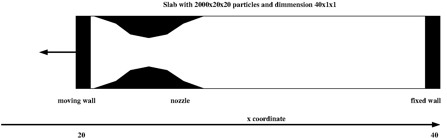
• Now create the setup:
  • First assume a wall at the right end of the slab.
  • Second create a wall on the left end of the slab, which is moving to the left.
  • Create a symmetric nozzle (i.e., a reduction of the area in the y direction) at the left side of the slab (but leave some place for the initial position of the moving wall).
  • Now move all more to the right side, so that the left wall can safely move to the left.
  • Hint: Here a is sketch of the geometry:
    

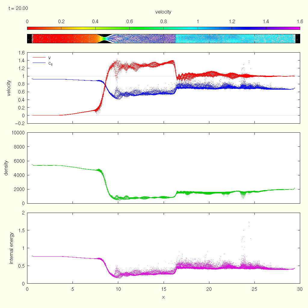
Now we can perform the simulation and analyze it.

• When compiling the code, do not forget to switch on SPH_BND_PARTICLES.
• Try to explain what is happening in the simulation.
• Is the gas at the beginning streaming through the nozzle (if not, why)?
• What happens to the gas on the opposite of the nozzle (and why)?
• Try to have a look at the temperature of the gas.
• What happens when the gas is finally flowing through the nozzle?

Programming goals for T7:

Producing initial condition with special boundary regions, especially we will

• learn how to create boundary regions in the initial conditions
• how to define special shapes and obstacles

Solution

A flow through a nozzle

• Again, extending the setup script from T06, combining with what we did in T03, we first create a 2000x20x20 slab and the place the different obstacles in it.
  • setup_nozzle.pro in IDL
  you should get something like shown below, where red dots indicate the defined boundary particles
  
• Example for the simulation
  
  • Examples for Config.sh and nozzle.param to be used.
  • show_nozzle.pro in IDL
  you should be able to obtain an animation like this and identify all the phenomena discussed in the experiment from above
  
• Example using Fortran and gnuplot:
  • ifort -g -traceback -check all -fpe0 -o nozzlesetup nozzlesetup.f90
    (this uses glass.txt from T04)
  • ./nozzlesetup
  • gnuplot grid.plt (to check that the particle positions are set up correctly)
  • compile Gadget with LONG_X=30, LONG_Y=1, and LONG_Z=1 (and PERIODIC and NOGRAVITY)
  • run Gadget using nozzle.ic as the initial conditions file and output as the snapshot file base in the parameter file (and TimeMax = 20 (the time it takes the moving wall traveling at v = 1 to reach the end of the simulation volume) and TimeBetSnapshot = 0.05)
  • ifort -g -traceback -check all -fpe0 -o readsnap readsnap.f90
  • for file in output_???; do ./readsnap $file >$file.txt; done
  • gnuplot nozzle.plt
    (this requires ffmpeg, which is installed on our ltsp machines)
  • xine -l nozzle.mp4