T4: The Riemann Problem:
try it out on your own

Before the tutorials:

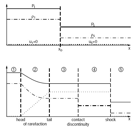
As discussed in the Lecture, the Riemann Problem is the key pillar of Eulerian hydrodynamics and can not be solved fully analytically. In the lecture, we solved a special case of it. So, start with this picture

taken from Simulation Techniques for Cosmological Simulations. Now, think about:

• How can we use the particle distributions from last time to initial conditions for the problem above?
• How are different densities represented?
• How can I verify the solution I get from the simulation?

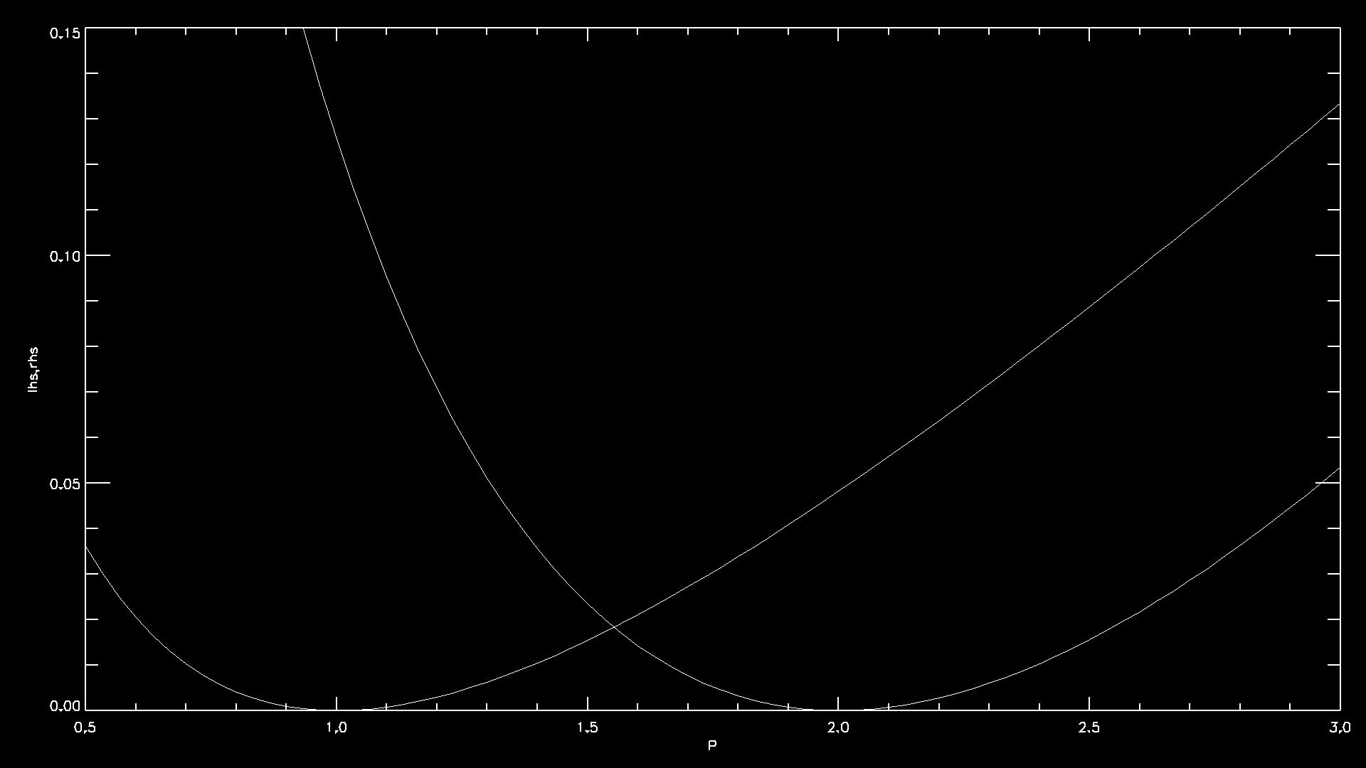
Also, remember that we had the equation

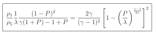
with

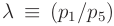
to solve to get the solution for the pressure at the contact discontinuity (so pressure in sector 3 and 4). Think about:

• How can you simply solve the this equation?
• How can i check it against the simulation performed?

During the tutorials:

You can start from the configuration of the code as obtained in T03 and collect some different particle distributions.

• Copy over the code and the parameter file as described in T03
• Copy over the Cubic Lattice you created in T03

You can now write a program to set up a long slab (along the x-axis) which resembles your initial conditions.

• Stack the basic particle files along the x-direction.
• Set the left and right state.

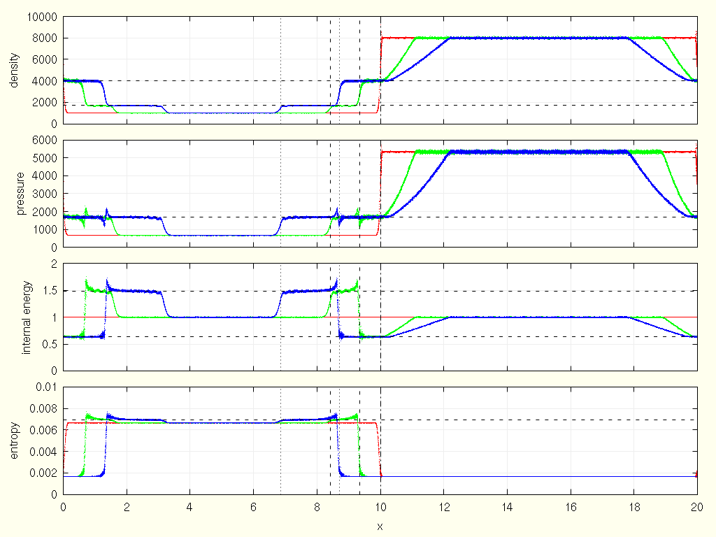
Now you can run the simulation.

• When compiling the code, do not forget to switch on PERIODIC and NOGRAVITY again. Also, you have to indicate the non-cubic form of the simulation domain by setting LONG_X=100, LONG_Y=1 and LONG_Z=1 in the Config.sh file before compiling.
• Set up the parameter file for the simulation, especially adapt DesNumNgb, TimeMax, InitCondFile, BoxSize and SnapshotFileBase.

Programming goals for T4:

Goal of this tutorial is that you learn better how to create non-uniform initial conditions.

Solutions

• Example(s) for initial conditions
  • cp $HOME/Hydro/grid_10x10x10 .
  • cp $HOME/Hydro/grid_12x12x12 .
• Examples for script to set up simulations
  • setup_slab.pro in IDL
• Example(s) for visualising the results
  • show_slab.pro in IDL
• You should see a movie like this
  
• To solve the Riemann problem you can plot the left hand side (lhs) and the right hand side (rhs) of the above equation to find P where the two are equal:
  
• Example using Fortran and gnuplot:
  • ifort -g -traceback -check all -fpe0 -o slabsetup slabsetup.f90
    (this uses glass.txt, which is a text version of the glass file with coordinates in the range of 0 . . . 1)
  • ./slabsetup
  • gnuplot grid.plt (to check that the particle positions are set up correctly)
  • compile Gadget with LONG_X=20, LONG_Y=1, and LONG_Z=1 (and PERIODIC and NOGRAVITY)
  • run Gadget using slab.ic as the initial conditions file and output as the snapshot file base in the parameter file, and BoxSize 1
  • ifort -g -traceback -check all -fpe0 -o readsnap readsnap.f90
  • ./readsnap output_000 >output_000.txt
  • ./readsnap output_010 >output_010.txt
  • ./readsnap output_020 >output_020.txt
  • gnuplot pressure.plt
  • gv pressure.ps