T0b: Introduction:
connecting, compiling, running, reading data

Before the tutorials:

As discussed in the Lecture, it is important to know the length scale on which the basic constituents of a medium interact. Start with the figure 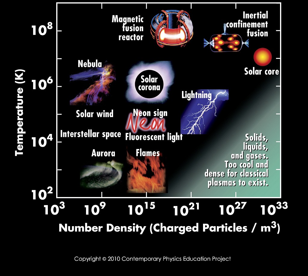to think about and work out the following:

• Identify the astrophysical systems in this plot and think about what they are.
• What is the physical size of these systems?
• What is the physical state of the matter in these systems and why?
• Can you place some more astrophysical systems on this plot?
  Try at least to place the intra-cluster medium and some special regions within the Milky Way.
• Can you compute the mean free path between particles for some of the astrophysical systems you have in the plot?
• Compare this mean free path to the size of the system.
• Many(?) of these system will have charged particles. Do they have magnetic fields?
  If so, how big are they and what is the expected gyro radius of the particles?

During the tutorials:

You will all use a shared computational resource (a USM compute cluster) and will use a job scheduling system to share the resources!

To do each tutorial, you need to follow some basic steps:

Step 1:

Connect to our machines (i.e., mpusm06.usm.uni-muenchen.de) and change into the directory you created (remember the individual steps done in T0a)

Step 2:

Set up the numerical experiment. (Note that there can be several numerical exercises in each tutorial.) To do so, there are 5 fundamental steps:

Step 2a:

Make a new directory for your experiment.

Step 2b:

Get the code.

Step 2c:

Get the configuration file (Config.sh) for the code.

Step 2d:

Get the parameter file (e.g., box.param) for the simulation.

Step 2e:

Get the job queue submission script (e.g., runme.sh).

Step 3:

Perform the numerical experiment. To do so, there are 6 fundamental steps:

Step 3a:

Modify the configuration file (Config.sh) for the code, i.e., change into Hydro-OpenGadget3 and set/unset the options needed for the current experiment.

Step 3b:

Compile the code (change into Hydro-OpenGadget3 and type make).

Step 3c:

Create the initial conditions for the numerical experiment you want to perform. Here you can use the programming language of your choice. We will always give examples, but not in all languages. So please get familiar with how to do this step. This is basically defining the domain and initialization of your experimental setup.

Step 3d:

Modify the parameter file (typically something.param) by specifying the details of your current experiment (i.e., give the parameter values tailored to the exact experiment).

Step 3d:

Prepare the submission script (e.g., runme.sh) for the experiment (that is, specify the name and the resources you want to use).

Step 3e:

Submit the script to the queuing system.

Step 4:

Visualize the results of the numerical experiment (when the simulation has finished running).

Repeat steps 2, 3, and 4 for the next experiment.

Step 1: Connecting

• Make sure that you have installed the VPN client and start it.
• Remember the individual steps done in T0a needed to connect to our compute cluster:
  • If you have a working X11 environment running on your Laptop (e.g., on a Linux operating system or with Cygwin/XQuartz installed on your Windows/macOS laptop), then you can just follow the steps as done last time:
    • Start the X server from a Cygwin terminal (X -multiwindow).
    • Start a second terminal, and
      • do not forget to specify the display number (export DISPLAY=:0)
      • ssh -4 -Y hydro@mpusm06.usm.uni-muenchen.de
  • If you do not have a working X11 environment:
    • On Windows: install the Cygwin package.
    • On macOS: install the XQuartz package.

Step 2: Setup

• As a first step, create your own directory (if not already done last time) and a subdirectory for this tutorial, and change into this directory:
  • mkdir MyName
  • mkdir MyName/Tutorial00
  • mkdir MyName/Tutorial00/Experiment1
  • cd MyName/Tutorial00/Experiment1
• As a second step, get a copy of the simulation program into your directory:
  • git clone https://gitlab.lrz.de/MAGNETICUM/Hydro-OpenGadget3
• As a third step, copy the configuration file for the code into your directory:
  • cd Hydro-OpenGadget3
  • cp $HOME/Hydro/Config.sh .
  • cd ..
• As a last step, copy the parameter file and the job submission script into your directory:
  • Copy the parameter file: cp $HOME/Hydro/box.param .
  • Copy the job submission script: cp $HOME/Hydro/runme.sh .

Step 3: Perform the numerical experiment

• (3a/b) Compile the simulation program:
  • module load compiler openmpi (this has to be run only once after you have connected to our machines).
  • cd Hydro-OpenGadget3
  • Modify the content of Config.sh as described for each experiment (for the first experiment, nothing to do).
  • make -j
  • cd ..
• (3c) Copy the initial conditions or write a small program which creates them.
  • As first step, just copy the already prepared initial conditions (cp $HOME/Hydro/box.ic .) and continue with (3d).
  • Later, after doing all the steps you can start here again and create the initial conditions yourself, before continuing with (3d):
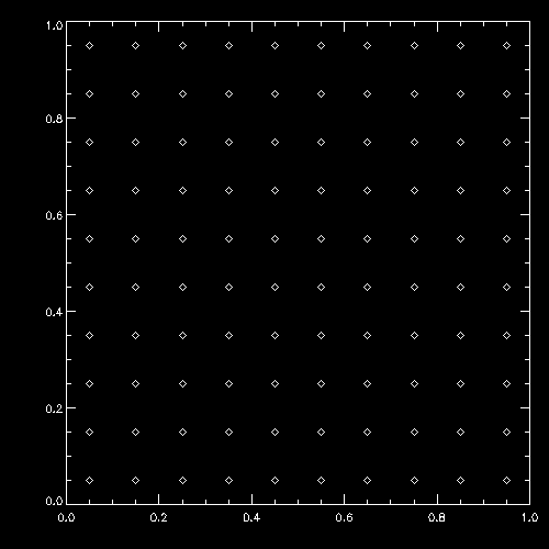
    Set up a cube of 10×10×10 particles in a region with the coordinates [0...1].
    Give a tiny velocity in the x direction and write the data into an initial conditions file box.ic.
    • Use the example in the IDL language:
      • cp $HOME/Hydro/IDL/Setup/*.pro .
      • idl -e setup_grid
    • or the example in the C/C++ language:
      • cp $HOME/Hydro/C/gadget_io.h .
      • cp $HOME/Hydro/C/setup_grid.c .
      • icx setup_grid.c
      • ./a.out
    • or the example in the Fortran language:
      • cp $HOME/Hydro/Fortran/gadget_io.f90 .
      • cp $HOME/Hydro/Fortran/setup_grid.f90 .
      • ifx gadget_io.f90 setup_grid.f90
      • ./a.out
    • or the example in the Python language:
      • cp $HOME/Hydro/Python/g3read.py .
      • cp $HOME/Hydro/Python/setup_grid.py .
      • cp $HOME/Hydro/Python/ic_header .
      • python3 setup_grid.py
    • or the example in the Julia language:
      • cp $HOME/Hydro/Julia/setup_grid.jl .
      • julia setup_grid.jl
• (3d) Modify the parameter file and the job submission script.
  • Modify the content of box.param as described for each experiment (for the first experiment, nothing to do).
  • Modify the content of runme.sh to match the requirements for the experiment (for the first experiment, please change the value of job-name to a unique string and choose the value 1 for both ntasks and cpus-per-task).
• (3e) Now actually perform the numerical experiment by running the hydro simulation:
  • sbatch runme.sh (this submits the job to the slurm scheduler system on the compute cluster).
  • You can check if your simulation is running by typing the squeue command.
  • You can see the progress of your simulation by typing tail slurm-[YOUR_JOB_ID].out.
  • Individual time instances of the whole simulated system are saved in files like snap_XXX.
  You can control how many cores are used by the program by setting
  • ntasks (the number of MPI ranks to use) to larger numbers.
  • cpus-per-task (the number of OpenMP threads each MPI task should use) to larger numbers.
  Note that on our systems the product of both should not exceed 32.

Step 4: Visualize the results of the numerical experiment

• (4a) Write a small program to display the result of the first output:
  • Use the example in the IDL language:
    • cp $HOME/Hydro/IDL/Show/*.pro .
    • idl -e show_single
    • display frame_000.png
  • or the example in the C/C++ language:
    • cp $HOME/Hydro/C/gadget_io.h .
    • cp $HOME/Hydro/C/show_single.* .
    • icx show_single.c
    • ./a.out >data.txt
    • gnuplot show_single.plt
  • or the example in the Fortran language:
    • cp $HOME/Hydro/Fortran/gadget_io.f90 .
    • cp $HOME/Hydro/Fortran/show_single.* .
    • ifx gadget_io.f90 show_single.f90
    • ./a.out >data.txt
    • gnuplot show_single.plt
  • or the example in the Python language:
    • cp $HOME/Hydro/Python/g3read.py .
    • cp $HOME/Hydro/Python/show_single.py .
    • python3 show_single.py
    • display frame_000.png
  • or the example in the Julia language:
    • cp $HOME/Hydro/Julia/show_single.jl .
    • julia show_single.jl
    • display frame_000.png

• (4b) Extend the program to create a time evolution of the result:
  • Use the example in the IDL language:
    • cp $HOME/Hydro/IDL/Show/*.pro .
    • idl -e show
    • xv frame_0*.png -wait 0.1 -wloop
  • or the example in the C/C++ language:
    • cp $HOME/Hydro/C/gadget_io.h . (if not already done in step 3c)
    • cp $HOME/Hydro/C/show.* .
    • icx show.c
    • ./a.out snap_* >data.txt
    • gnuplot show.plt (press enter to go forward)
  • or the example in the Fortran language:
    • cp $HOME/Hydro/Fortran/gadget_io.f90 . (if not already done in step 3c)
    • cp $HOME/Hydro/Fortran/show.* .
    • ifx gadget_io.f90 show.f90
    • ./a.out snap_* >data.txt
    • gnuplot show.plt (press enter to go forward)
  • or the example in the Python language:
    • cp $HOME/Hydro/Python/g3read.py . (if not already done in step 3c)
    • cp $HOME/Hydro/Python/show.py .
    • python3 show.py
    • ffplay -loop 0 basic_animation.mp4
  • or the example in the Julia language:
    • cp $HOME/Hydro/Julia/show.jl .
    • julia show.jl
    • animate scatter.gif

Programming goals for T0:

Goal of this tutorial is that you learn how to use commands in a unix shell,
how to compile and execute a program,
how to write a simple program (concept of “main”),
how to define variables and calculate values in a program,
how to perform output from a program,
how to start a simulation, and
how to plot the results.

Running on other platforms

If you want to do the tutorials on an other platform (like your own PC), you need to have at least a C++ compiler installed and an MPI environment. In addition you need to have the gsl library available, plus whatever you want to use for creating your plots.

Further information