T3: Density estimates:
particle distributions and kernels

Before the tutorials:

As discussed in the Lecture, kernel density estimates are the key pillar of smoothed particle hydrodynamics (for an general overview on density estimations, see this survey of existing methods). Kernel density estimators are used to smooth a discretized distribution of tracer particles to obtain continuous fields needed in hydrodynamics. Therefore it is important to understand the intrinsic properties of such kernel density estimators.
Start with this picture: taken from this paper (figure 1) and think about:

• How are the simple particle distributions (especially Cubic Lattice and Hexagonal Close Packing) defined?
• What is a Glass distribution?
• How can you extend the program from T0b you used to set up a Cubic Lattice to the Hexagonal Close Packing case?

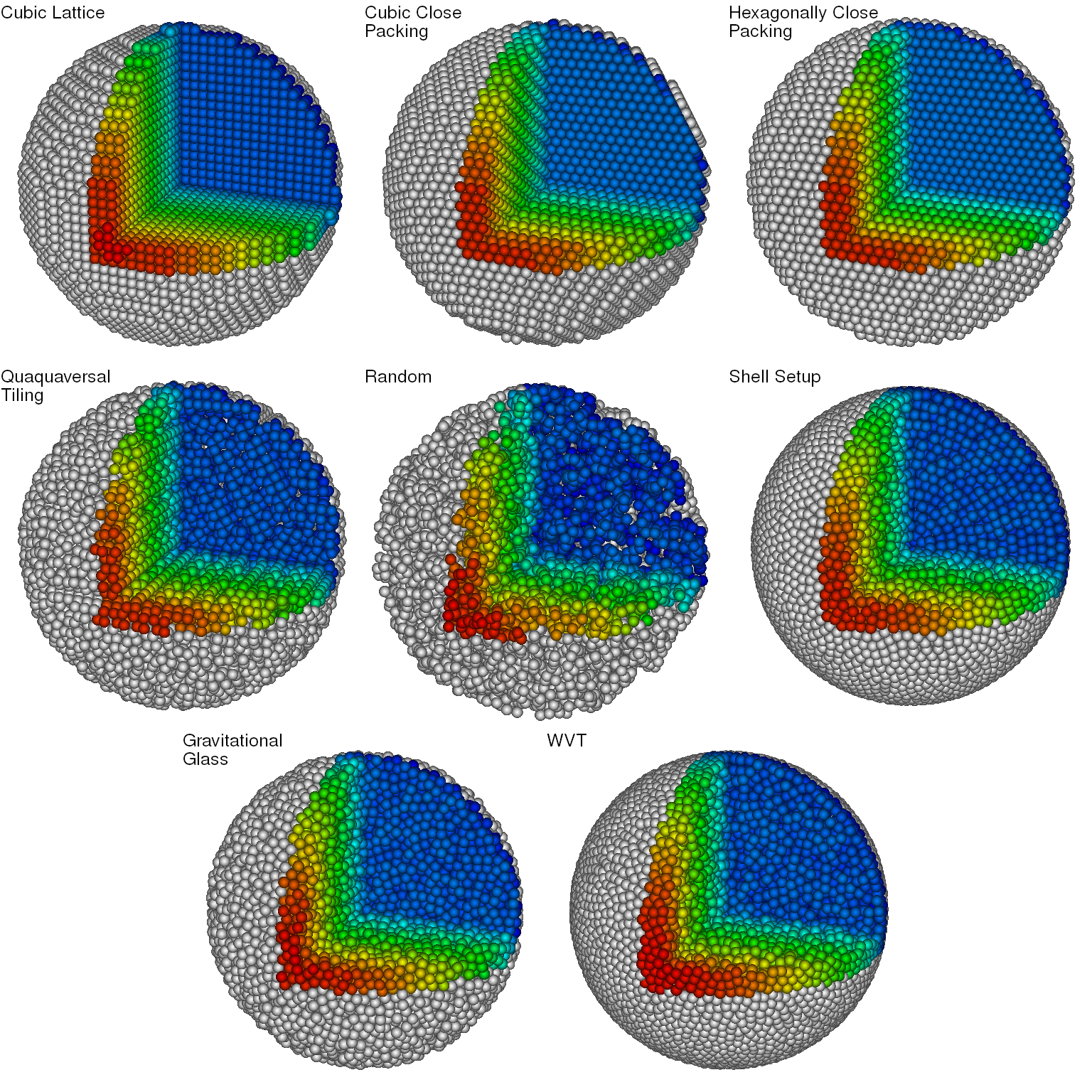
The global properties of kernels have a significant impact on the performance of SPH. Make yourself familiar with some common choices of kernels (especially the spline and Wendland ones), as summarized in table 1 and figure 1 of this article.

During the tutorials:

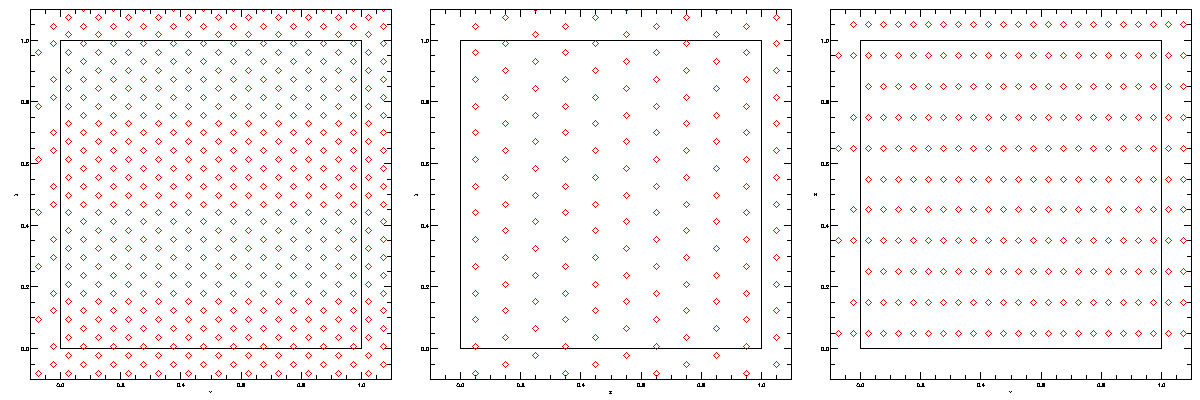
You can start from the configuration of the code as obtained in T0b and collect some different particle distributions.

• Copy over the code and the parameter file as described in T0b Step 2
• Copy over the Cubic Lattice you created in T0b Step 3
• Copy over the Glass file provided: cp $HOME/Hydro/glass_10x10x10 .
• For people who want to look at something special: Take the setup_grid from T0b Step 3c and modify it so that you get random positions of particles within the box.

You can now run the program using different kernels and different neighbor numbers. Keep in mind that you do not need to run the simulation for a very long time, basically you just need one output file. So set the TimeMax as well as the TimeBetSnapshot parameter in the box.param file to 0.5. Every setup/combination of kernel, number of neighbors, and initial particle distribution is an independent simulation you need to perform. To do so, you can:

• Specify the kernel to be used in the Config.sh file. Choices are STANDARD_KERNEL (i.e., the standard, Cubic Spline kernel), alternatively you can set QUINTIC_KERNEL, WENDLAND_C2_KERNEL, WENDLAND_C4_KERNEL, or WENDLAND_C6_KERNEL in the Config.sh file to select different kernels. Only one of the above settings can be set. Do not forget to re-compile after changing the kernel.
• To change the number of neighbors used, change the value for the DesNumNgb parameter in the box.param file, and re-run the simulation.
• To change the particle distribution to be used, change the name given for the InitCondFile parameter in the box.param file to the names of the different distributions and re-run the simulation.

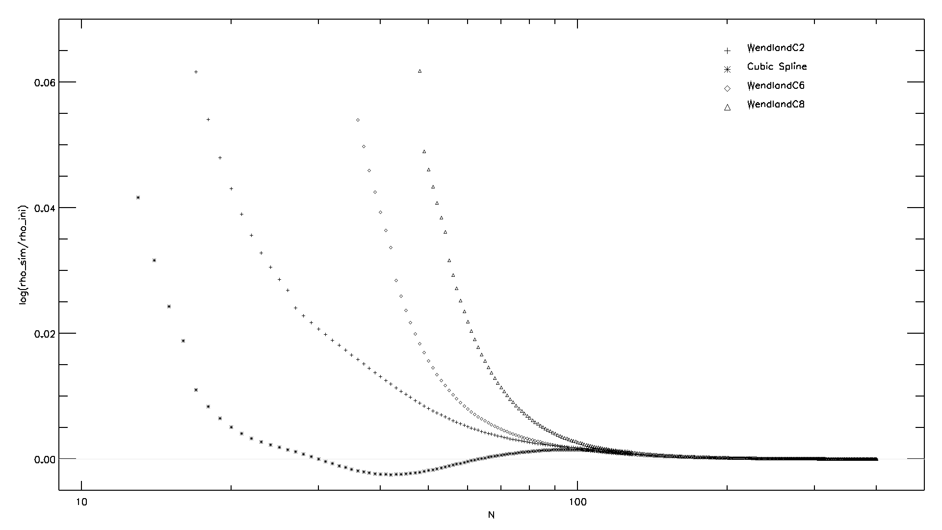
Now you can compare the resulting densities for the different simulations you produced. You can read the density ("RHO ") for all particles within the different simulations and compute the mean and the standard deviation, compared to the true density used to create the initial conditions. You can do this step by step:

• Plot the distribution of densities for all particles in one simulation.
• Compute the mean, median and the width of the distribution. Note down the values, together with the configuration used.
• Repeat this for the different choices of kernels, number of neighbors and initial particle distributions.
• Do some simple plots comparing these values for your different choices.
• Try to produce a figure similar to figure 3 of the above article.

Programming goals for T3:

Goal of this tutorial is that you learn better how to change the setup of the simulation and parameters.
What do you have to change to get only one output for each simulations?
Can you create a script to run the test with varying parameters?
How to produce a plot with multiple lines from different simulations?
How to produce one graph from the result of different simulations?

Solutions

• Example(s) for initial conditions
  • cp $HOME/Hydro/grid_10x10x10 .
    Make sure you are using BoxSize 1 in the parameter file!
  • cp $HOME/Hydro/packed_12x12x12 .
    Make sure you are using BoxSize 1 in the parameter file!
  • cp $HOME/Hydro/glass_10x10x10 .
    Make sure you are using BoxSize 1 in the parameter file!
• Example for scripts to read density and compute mean and variance:
  • Python language: python3 print_values.py^{Updated 2024-11-12}
• Examples for script to run simulations
  • parameterfile^{Updated 2024-11-12} with placeholders
  • shell script to run several simulations
• Example(s) for visualizing the results
  • Use the example in the IDL
    • idl -e show_kernels
  • Use the example in the Fortran language and gnuplot
    • ifx -g -traceback -check all -fpe0 -o meandensity meandensity.f90
    • bash runsims
    • gnuplot meandensity.plt
    • gv meandensity.ps
    • gnuplot density.plt
• You should see an image like this, with measured bias of the density estimate:
• Examples for script to set up a packed lattice
  • close_packed_lattice_new.pro in IDL