T01: Introduction:
connecting, compiling, running, reading data

Before the tutorials (science part):

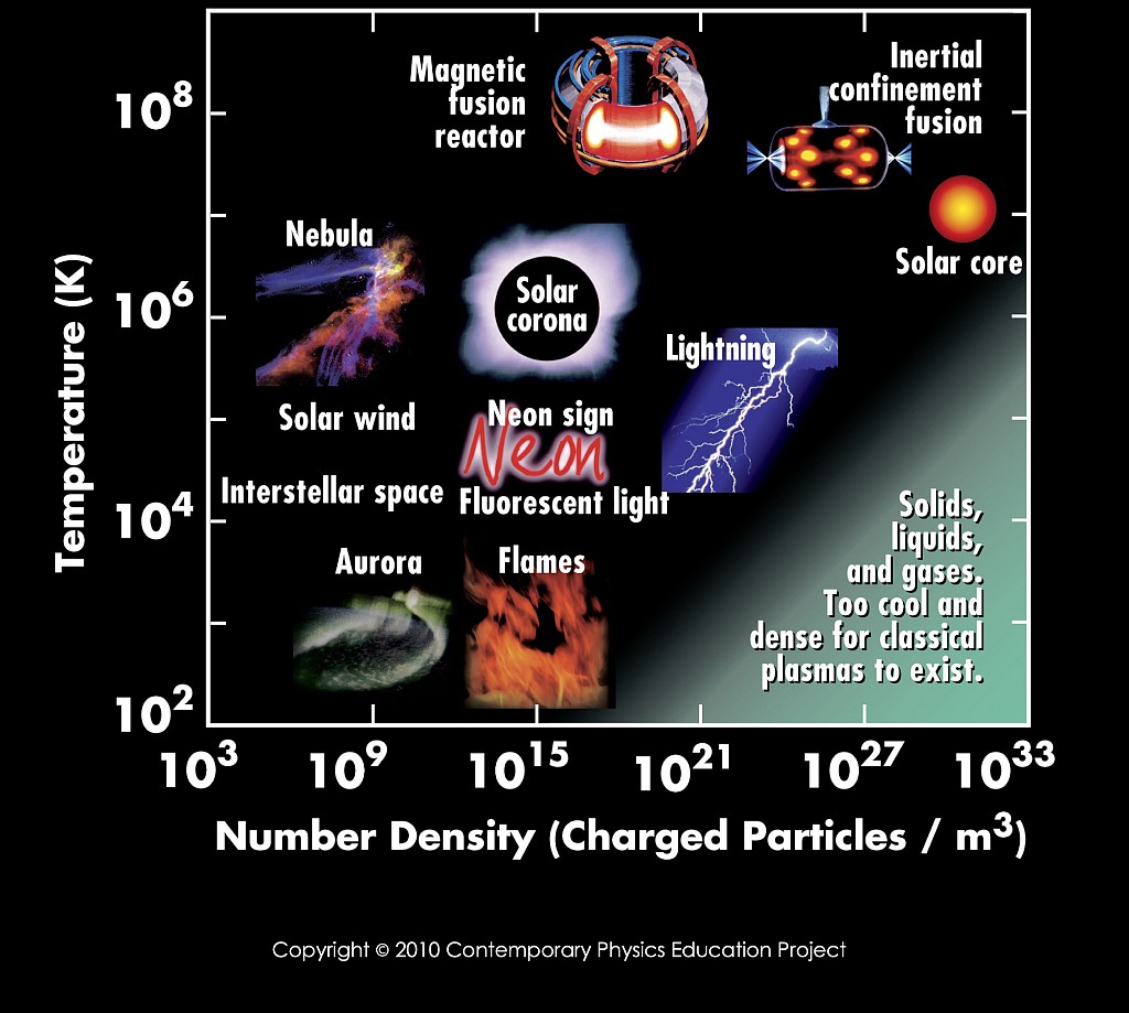
As discussed in the Lecture, it is important to know the length scale on which the basic constituents of a medium interact. Start with the figure to think about and work out the following:

• Identify the astrophysical systems in this plot and think about what they are.
• What is the physical size of these systems?
• What is the physical state of the matter in these systems and why?
• Can you place some more astrophysical systems on this plot?
  Try at least to place the intra-cluster medium and some special regions within the Milky Way.
• Can you compute the mean free path between particles for some of the astrophysical systems you have in the plot?
• Compare this mean free path to the size of the system.
• Many(?) of these system will have charged particles. Do they have magnetic fields?
  If so, how big are they and what is the expected gyro radius of the particles?

Before the tutorials (preparational part):

To make things as easy as possible for the numerical experiments, we prepared a mechanism so that you can run the numerical experiments on your laptop with minimal configuration efforts. We therefore prepared a docker image for you which you can run on your laptop to have the according environment.

So here some first steps to prepare:

• Get familiar with the basics of Unix like command line. How to create a folder, change directory, copy files, etc.
• Get familiar with how to edit a simple asci file with vi
• Install Docker Desktop on your laptop (see docker installation)
• Read the instruction for the docker files our git lab repo
• Download the .tar file of the container you need for your system an place it in an extra work folder.

During the tutorials:

You can perform all tasks within your docker session and access the results from outside.

To do each tutorial, you need to follow some basic steps:

Step 0:

(only need to be done once)

Open a comandline shell (e.g. xterm if you have Linux/Mac or PowerShell if you have Windows)

Go to the work folder where you downloaded the container

Prepare the container (e.g. docker load -i opengadget3-container-XXX.tar, replace the XXX with what you need on your system)

Step 1:

Start your docker session (i.e. docker run -it -v .:/mnt --name opengadget3_container opengadget3:XXX)

Create a new directory for each of the experiments when you perform one. If you do this under the /mnt then it is visible from outside the container. (e.g. first mkdir /mnt/T01, then cd /mnt/T01)

Step 2:

Set up the numerical experiment. (Note that there can be several numerical exercises in each tutorial.) To do so, there are 5 fundamental steps:

Step 2a:

Make a new directory for your experiment, as done above.

Step 2b:

Get the code, e.g. do cp -r ~/OpenGadget3 . within the directory for your tutorial.

Step 2c:

Copy the configuration file (Config.sh) into the code directory, e.g.
a) cd OpenGadget3
b) wget https://www.usm.uni-muenchen.de/~dolag/Hydro/Hydro/Config.sh
c) cd ..

Step 2d:

Get the parameter file (e.g., box.param) for the simulation, e.g.
a) wget https://www.usm.uni-muenchen.de/~dolag/Hydro/Hydro/box.param

Step 2e:

Get the initial condition file (e.g., box.ic), e.g.
a) wget https://www.usm.uni-muenchen.de/~dolag/Hydro/Hydro/box.ic

Step 3:

Perform the numerical experiment. To do so, there are 6 fundamental steps:

Step 3a:

Modify the configuration file (Config.sh) for the code, i.e., change into Hydro-OpenGadget3 and set/unset the options needed for the current experiment.
a) cd OpenGadget3
b) vi Config.sh (Note that this time you do not need to change anything)

Step 3b:

Compile the code, e.g.
a) source Build/Container_build.sh (Note that this has to be done only once for each session)
b) make -j
c) cd ..

Step 3c:

In some experiments, you might have to modify the initial conditions. In such case, we will provide additional informations how to do so later on. Here, in the first tutorial, you can just work with the box.ic file we provided and which you have downloaded in step 2e before.

Step 3d:

Modify the parameter file box.param to match the requironments of the current tutorial, e.g.
a) vi box.param (Note that again, for this tutorial there is nothing to change)

Step 3e:

Run the simulation, e.g.
a) mpiexec -np 2 OpenGadget3/OpenGadget3 box.param
after the simulations finished, you should fine several files with the simulation output, e.g. snap_???, as well as many .txt files with additional information in your directory.

Step 4:

Visualize the results of the numerical experiment (when the simulation has finished running).
To do so, there are 3 fundamental steps:

Step 4a:

Download, create or modify an plotting script, e.g.
a) wget https://www.usm.uni-muenchen.de/~dolag/Hydro/Hydro/Python/show_single.py
b) vi show_single.py (Note that for the first step, there is nothing to change)

Step 4b:

Execute the python script, e.g.
a) python3 show_single.py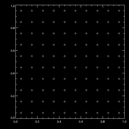
after this, you will have a picture file frame_000.png in your directory. As this is visible from outside the container, you can just watch it using your file browser.

Congratulations, you have for the first time runned a full cycle of setting up, unnimng and analyzing a simulation. Now get a little bit more familiar with some details of the steps.

Step 5: Improvising on Step 4a, How to do a simple plot

Have a more detailed look at the plotting script show_single.py which is kept quite simple. You can identify the line where the output file snap_000 is selected, and where the positions pos are read from the file. From the scatter plot command you can see, that pos is an array for all particles (first index) and the second index with encodes the x,y and z components. From the reading you can see that the label for the positions is "POS ".

• Step 5a: How to make a different plot
  

  Now you can try to read other vales of the particles from the file. You can try to use the velocity ("VEL ") which has three components like the positions before, or some scalar values like the density ("RHO "), the internal energy ("U ") or the smoothing length of each particle ("HSML"). Names are always filled with SPACE so that they have 4 characters. Now you can experiment with different kind of scatter plots.

• Step 5b: How to make a movie
  
  • wget https://www.usm.uni-muenchen.de/~dolag/Hydro/Hydro/Python/show.py
  • python3 show.py
    after this, you will have a movie file basic_animation.mp4 in your directory. As this is visible from outside the container, you can just watch it using your file browser.
  

Step 6: Improving on Step 3c, How to create your own initial condition

Initial conditions a basicly exactly the same files than the simulation output. They just contain all intrinsic properties (including the spacial distribution) of all SPH particles in the simulation. Starting from an empty template file ic_header we can just define arrays for the basic properties of the particles and assign them to define the geometry and setup of the experiment we want to do. As soon as we have done this, we can create a new box.ic file and do simulation based on this initial condition file.

So here an example, how to create the initial conditions for the problem we did before:

• Step 1: Get an example script and a template header
  • wget https://www.usm.uni-muenchen.de/~dolag/Hydro/Hydro/Python/setup_grid.py (This is an example script)
  • wget https://www.usm.uni-muenchen.de/~dolag/Hydro/Hydro/Python/ic_header (This has to be done only once to have the template file)
  • vi setup_grid.py (Let's have a look at the code, but nothing to change at the moment)
  • python3 setup_grid.py
    After this, you should have a new box.ic file in your directory.
• Step 2: Have a look at the setup_grid.py and see if you can find where the velocity in x-direction is set. Can you set it in the y-direction instead?
  • vi setup_grid.py (Now change the direction of motion in the initial conditions)
  • python3 setup_grid.py>
    After this, you should have a new box.ic file in your directory. Now you can re-run the simulations (Step 3e) and then watch how it looks different (Step 5b) than before.

Programming goals for T01:

Goal of this tutorial is that you learn how to use commands in a Unix shell,
how to compile and execute a program,
how to create initial condition,
how to start a simulation, and
how to plot the results.

Further information