Next: Atomic Models Up: Realistic Models For Expanding Previous: Introduction

The Concept of Radiation Driven Winds

Figure 3: Schematic sketch of the basic equations of stationary radiation-driven wind theory (see text).

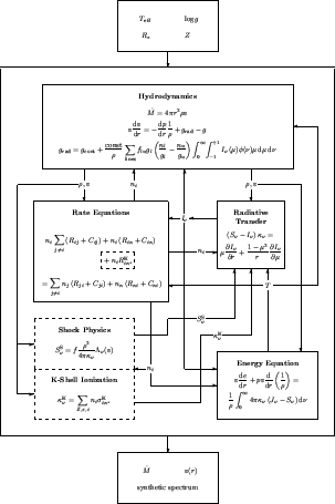$\begin{figure} \centerline {\hbox{ \psfig{file=06-concept.ps,width=14.cm}}}\end{figure}$

The concept of our expanding-atmosphere model calculations is based on the homogeneous, stationary, and spherically symmetric radiation-driven wind theory initially outlined by Lucy & Solomon (1970) and Castor, Abbott & Klein (1975). This concept turned out to be adequate for the analyses of hot-star spectra (see Fig. 2) and in spite of its restrictive character we are confident that in general it correctly describes the time-average mean of the spectral features. Fig. 3 gives an overview of the physics to be treated, and in the following we will briefly discuss the characteristic features of the system and describe our model approach. (A comprehensive discussion of most points is found in Pauldrach et al. 1994a.)

The principal features are:

The hydrodynamic equations are solved for pre-specified values of the stellar parameters T_eff, log g, R_*, and Z (abundances). The crucial term is the radiative acceleration g_rad, which has contributions from continuous absorption, scattering, and line absorption (the last term is calculated by summing the contributions of lines selected from our list containing more than 2500000 lines).
The occupation numbers for up to 5000 levels are determined by the rate equations containing collisional (C_ij) and radiative (R_ij) transition rates. For the calculation of the radiative bound-bound transition probabilities the Sobolev plus continuum method is used (cf. Hummer & Rybicki 1985, Puls & Hummer 1988, and Taresch et al. 1997). Low-temperature dielectronic recombination is included (in total 20000 transitions) and Auger ionization due to K-shell absorption (considered for C, N, O, Ne, Mg, Si, and S) of soft X-ray radiation arising from shock-heated matter is taken into account.
The spherical-transfer equation which yields the radiation field in the observers frame at up to 3500 frequency points at every depth point, including the thermalized layers where the diffusion approximation is applied, is correctly solved for the total opacities ( $\kappa_{\nu}^{}$ ) and source functions (S $\scriptstyle \nu$ ). Hence, the strong EUV line blocking which acts mainly between 228Å and 911Å, and which constitutes the ionizing flux and influences the ionization and excitation of levels, is properly taken into account (see Section 3).
Moreover, the emission from shocks arising from the non-stationary, unstable behaviour of radiation-driven winds (see, for instance, Prinja & Howarth 1986) is, together with K-shell absorption, also included in the radiative transfer. For the calculation of the shock source function ( S $\scriptstyle \nu$ ^S) we did not directly use the results of the theoretical investigation of time-dependent radiation hydrodynamics that describes the creation and development of shocks (cf. Owocki, Castor & Rybicki 1988; Feldmeier 1995, 1997XXX; note that the reliability of these calculations was recently demonstrated by a comparison to ROSAT observations (cf. Feldmeier et al. 1997)). Instead, the shock source function was incorporated in a preliminary way on the basis of an approximate calculation where the volume emission coefficient ( $\Lambda_{\nu}^{}$ ) of the X-ray plasma is calculated using the Raymond & Smith (1977) code (cf. Hunsinger 1993) and the velocity-dependent post-shock temperatures and the filling factor (f) enter as fit parameters (cf. Pauldrach et al. 1994b).
The temperature structure is determined by the microscopic energy equation which, in principle, states that the luminosity must be conserved. In our present calculations line blanketing effects which reflect the influence of line blocking on the temperature structure are taken into account (see Section 3).
The iterative solution of the total system of equations then yields the hydrodynamic structure of the wind (i.e.,the mass-loss rate [ $\dot{M}$ ] and the velocity structure [v(r)]) together with synthetic spectra and ionizing fluxes.

As our present treatment of O-star atmospheric models is of course not free from approximations - in common with all other approaches to the theory (e.g., Schaerer & de Koter 1997; Hillier & Miller 1997) - we will emphasize the crucial points which either have important consequences or which still imply some uncertainties for our model calculations in more detail.

Table 1: Summary of Atomic Data. Columns 2 and 3 give the number of levels in packed and unpacked form; in columns 4 and 5 the number of lines used in the rate equations and for the line-force & blocking calculations are given, respectively.

Ion

Number of

Number of

Total non-LTE

Total

packed levels

levels

lines

lines

CIII

50

90

520

4407

CIV

27

48

103

229

NIII

40

80

356

16458

NIV

50

90

520

4201

NV

27

47

104

229

OIII

50

118

582

25511

OIV

44

90

435

17933

OV

50

88

524

4336

NeIII

38

78

319

857

NeIV

50

113

577

4470

NeV

50

110

534

2664

SiIII

50

88

480

4044

SiIV

25

45

90

245

SiVI

50

122

596

3889

SIII

14

28

32

190

SIV

13

23

22

70

SV

14

26

17

82

SVI

18

32

59

142

ArIII

13

26

21

1912

ArIV

11

23

22

398

ArV

40

96

328

3007

ArVI

42

93

400

1335

FeIII

50

122

246

199484

FeIV

45

126

253

14346

FeV

50

122

442

10831

FeVI

50

104

452

11533

NiIII

40

112

281

131508

NiIV

50

148

528

11979

NiV

41

95

70

9207

NiVI

45

128

253

10821

Subsections

Atomic Models

Next: Atomic Models Up: Realistic Models For Expanding Previous: Introduction

1999-10-16